In my last post, I discussed Runge-Kutta-Nyström (RKN) methods, and a generic strategy for turning any Runge-Kutta method into an RKN method. The focus was more on the simplest way to do so, rather than the best way.

Today I found that there’s a way of improving cumulative error from O(h^3) to O(h^4), with very little additional compute required.

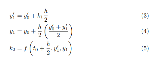
Let’s examine a simplification I glossed over – when calculating k_2, we know y’_n and y’_1. We can get an estimate for y_1 by integrating the polynomial which meets the conditions f(0)=y’_n and f(t_f)=y’_1. This is just the trapezoidal rule.

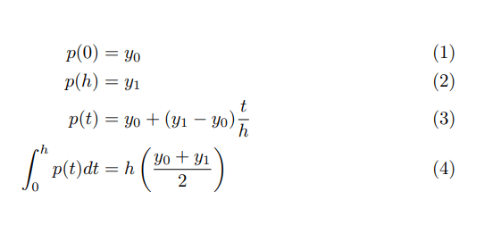
This takes two obvious pieces of information – we know the slope of y at the beginning and end of each interval for which we’re estimating the change in y. However, it ignores that we also know the acceleration of y. That is, we have a third initial condition:

Thus, we need a quadratic to represent the general function which meets all of these criteria:

Integrating gives:

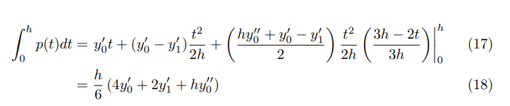
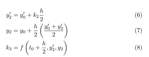
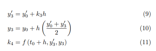
So all we need to do is replace our use of the trapezoidal rule with this quadratic rule. Recall that by definition, k_1 = y”_0, so it appears in every y_i estimate.

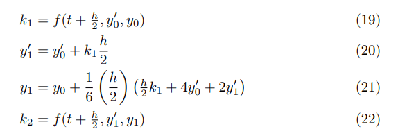
We repeat this pattern to calculate k_3:

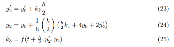
and k_4:

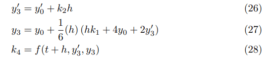
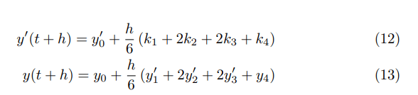
Then, we finish our estimation of y_n+1 and y’_n+1 as before:

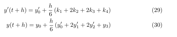
The impact on the accuracy of RKN algorithms is staggering. Using the same differential equation as last post, I’ve re-run the calculation of cumulative error. In the below table, “Before” denotes the algorithm from the previous post, with the trapezoidal rule, and “After” is with the quadratic rule.

Steps	Before Error(y)	After Error(y)		Before Error(y’)	After Error(y’)
1	1.484 E-3	3.438 E-3		1.593 E-2	4.681 E-4
10	7.797 E-6	3.529 E-7		2.282 E-5	7.484 E-8
100	8.967 E-9	3.486 E-11		2.366 E-8	7.914 E-12
1000	9.086 E-12	2.664 E-15		2.375 E-11	5.773 E-15

We’ve improved the cumulative error of the algorithm from O(h^3) to O(h^4) – an entire factor of h! The additional performance cost is tiny – at most an increase of 10% for trivial second-order differential equations – so this modification to the original algorithm should always be worth it.

You can recreate the results of this blog post by checking out v0.1.3 of my diffeq-go repository and running:

diffeq-go$ go run cmd/validate/validate.go

Alternative Title: How to turn any Runge-Kutta method into a Runge-Kutta-Nyström algorithm.

Differential equations describe everything from how populations grow with time to how waves flow through the ocean. While a few have nice analytic expressions, many do not – think the three-body problem or the Navier-Stokes equations. This isn’t a matter of the algebra being difficult – for many cases it can be shown that no such “nice” solution exists. In these cases we turn to computers and numerical methods.

Runge-Kutta methods are a family of numerical methods for solving first-order differential equations:

They offer startling performance and quality gains over the Euler Method. A fourth-order Runge-Kutta method can easily produce solutions many orders of magnitude more precise, all while requiring a fraction of a percent of the computing power the Euler Method demands.

However, Runge-Kutta methods have several limitations for studying complex systems:

1. They are limited to first-order differential equations.
2. They produce solutions for differential equations of a single variable.

I’m going to tackle the first of these two problems with a different family of solvers – Runge-Kutta-Nyström (RKN) methods.

Runge-Kutta-Nyström methods have a single sentence on Wikipedia describing them – a mere 20 word side-note in an article of over 3,000 words. There are several thousand articles on RKN methods on Google Scholar, many of them specialized and with little explanation of the basics – such as how to implement them or use them. While specialized RKN methods are very useful in the use cases they were developed for, they are not illustrative.

Fortunately, we don’t need to perform (as much of) the work required to develop RKN methods – we can take any existing Runge-Kutta method and adapt it to be an RKN method.

Let’s begin with a well-known Runge-Kutta method – RK4. However, we’ll write it as if we were solving a differential equation for y” in terms of y’. We want to produce an algorithm which solves this equation:

The modification for the expression for k_1 is straightforward – expand it to include the initial value of y:

Now, we define our estimate for y’ which we’ll use to compute k_2, y’_1 and then use the trapezoidal rule to extrapolate an estimate for y for estimating k_2.

Similarly for k_3:

And finishing the pattern, we get

And then plug in as we would for RK4 to produce our results:

Importantly, note that we use the RK4-weighting on estimating both y’ and y – the trapezoidal rule was only for calculating our k-values.

That’s it. This RKN4 algorithm produces results with cumulative O(h^3) error instead of the normal O(h^4) we expect for RK4, but this is unsurprising as we’re integrating slope, which has step-wise O(h^4) error.

The following table records the decrease in cumulative error in while evaluating y”(t) = 0.5 y'(t) + 0.5 y(t) with initial conditions y'(0) = y(0) = 1 and t_f = 1.0.

Steps	Error(y)	Error(y’)
1	1.484 E-3	1.593 E-2
10	7.797 E-6	2.282 E-5
100	8.967 E-9	2.366 E-8
1000	9.086 E-12	2.375 E-11

Performance-wise, for trivial differential equations RKN4 requires about 50% more compute time than a similar first-order equation evaluated with RK4. As RKN4 requires the same number of function evaluations as RK4, this difference is smaller for more involved equations.

I’ve published the code I developed for this blog post on GitHub. My results can be recreated by checking out tag v0.1.2 and running “go run cmd/validate/validate.go”.